How to Make a Gantt Chart in Google Sheets
Follow the steps below to quickly create a Gantt chart using Google Sheets. A Gantt chart in Google Sheets can help you track your project progress and keep an eye on key milestones.
To learn more about Gantt charts, including their history and why they’re a beneficial tool for project management, visit this article about Gantt charts. For even more ways to create a Gantt chart in different forms, including Microsoft Excel, Apple Pages, Apple Numbers, and Google Sheets, visit our comprehensive how-to article.
Open a New Google Sheet
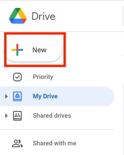
- On the Google Drive homepage, click the + New button.
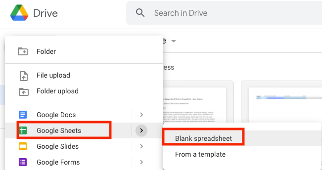
- Highlight Google Sheets from the dropdown, and click Blank Spreadsheet.
Transform your project details into an easy-to-read Gantt chart with Smartsheet
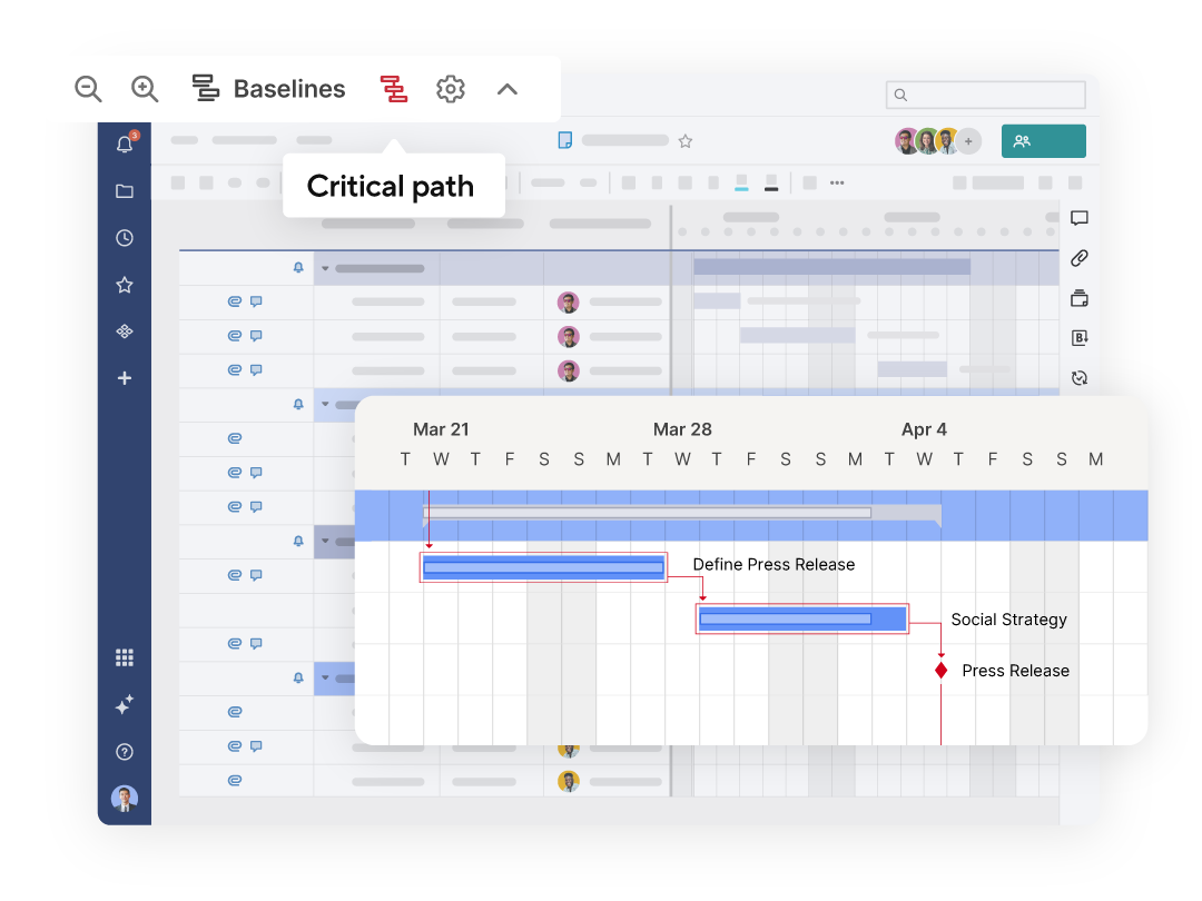
Smartsheet Gantt charts are a powerful tool for project planning, scheduling, and progress tracking. Display tasks across time with horizontal bars, view dependencies between tasks with ease, highlight important milestones, and identify a project's critical path to prioritize essential tasks.
Explore the full range of robust features when you try Smartsheet free for 30 days.
Input Project Data into Sheet
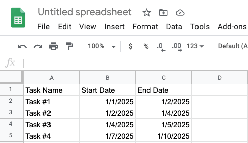
You’ll need to make two tables. The first table will serve as a template for the calculations you create in the second table.
- For the first table, label the columns as follows:
- Column A: Task Name
- Column B: Start Date
- Column C: Duration
Then label the cells as follows:
- Cell A2: Task #1
- Cell A3: Task #2
Continue until you have enough rows for each project task you want to appear on the Gantt chart. For example, if your project has four tasks, the table should have four rows in addition to the header row.
- Add corresponding start and end dates (in days) for each task.
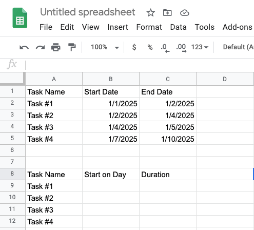
- Create the second table two to three rows below from the first one.In this example, we’re starting the second table in row 8. Label the cells as follows:
- Cell A8: Task Name
- Cell B8: Start on Day
- Cell C8: Duration
Pro Tip: The tasks in the Task Name column in the second table should be identical to those in the Task Name column in the first table. Copy and paste this information in the column below Task Name for the second table.
- Next, we need to figure out the start day for each task so that the bars accurately display the start date and duration.
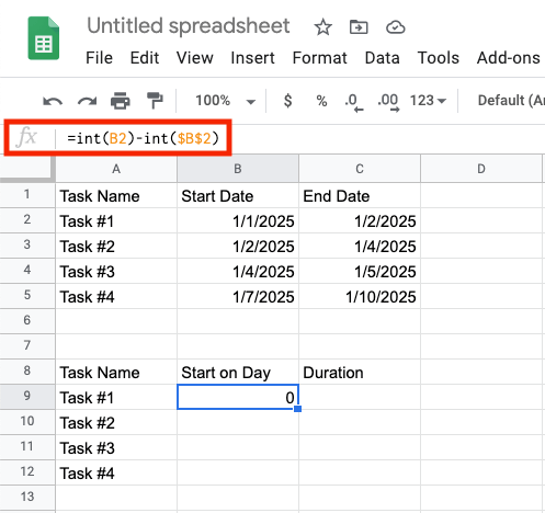
To determine the Start on Day value, find the difference between each task’s start date and that of the first task. In cell B9, input this formula:
=int(B2)-int($B$2)
Press Enter on your keyboard. The value will auto-populate in the cell.
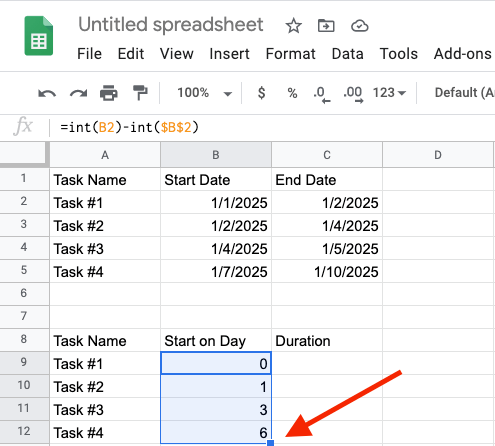
- For all the tasks in the Start on Day column, apply the same formula:
=int(B2)-int($B$2)
Click cell B9, and click and drag the small blue box in the bottom-right corner of the cell until you reach the last project task.
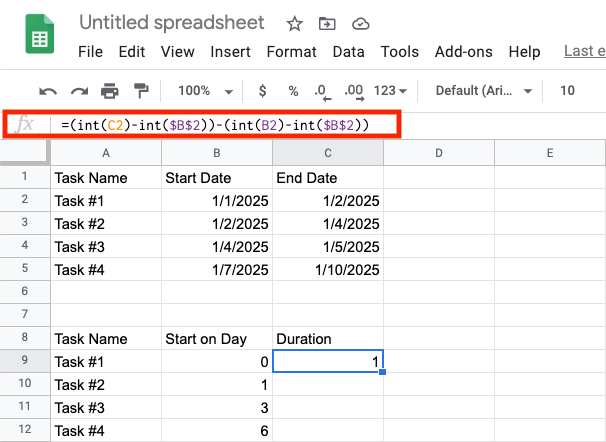
- Calculate the duration of each task. In the first cell of the Duration column (C9), input this formula:
=(INT(C4)-INT($B$4))-(INT(B4)-INT($B$4))
Press Enter on the keyboard. The value will auto-populate in the cell.
Pro Tip: The cell numbers might differ (e.g., C4 might be C10) depending on where you place project data in the sheet, but every other part of the formula should remain the same.
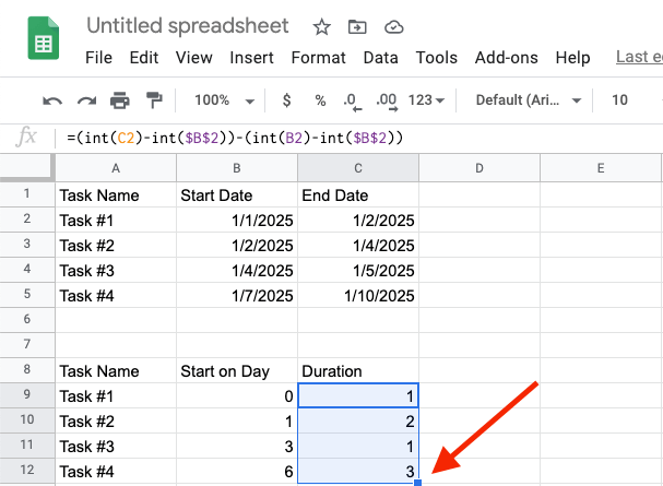
- For all tasks in the Duration column, apply the same formula:
=(INT(C4)-INT($B$4))-(INT(B4)-INT($B$4))
Click on cell C9, and click and drag the small blue box that appears in the bottom-right corner of the cell until you reach the last project task.
Create a Stacked Bar Graph
- Highlight the second table.
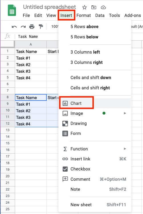
- Click Insert on the menu, then click Chart.
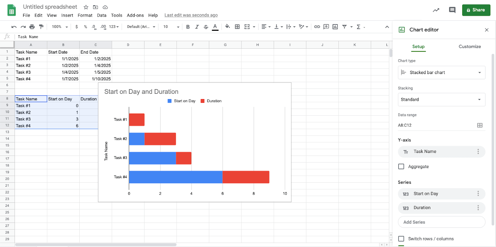
A stacked bar chart appears on the page.
Turn Your Stacked Bar Chart into a Gantt Chart
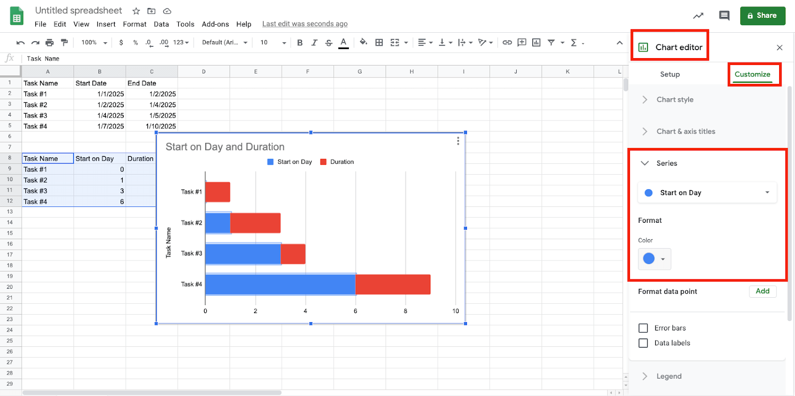
- Click on any Start on Day bar in the chart. This should highlight all the Start on Day bars.
- Configure the chart.
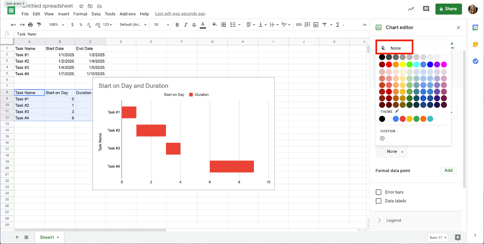
In the Chart editor panel on the right, click the Customize tab. Click Series, then click the dropdown menu and Start on Day. Click the Color button, then click None. The chart should now resemble a Gantt chart.
How to Customize a Gantt Chart in Google Sheets
It’s easy to customize everything from the title to the style of the bars on a Gantt chart. Follow the steps below to create 3D bars, remove the legend, change font colors, and more.
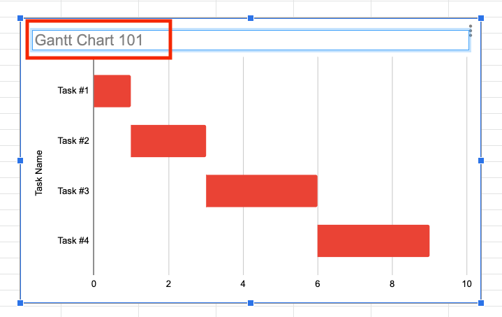
Update the Gantt Chart Title
- Double-click on the title at the top of the chart. Type in a new title for the project.
Customize the Gantt Chart Area
Follow these steps to change the appearance of your chart by adjusting the border color or making the bars pop in 3D.
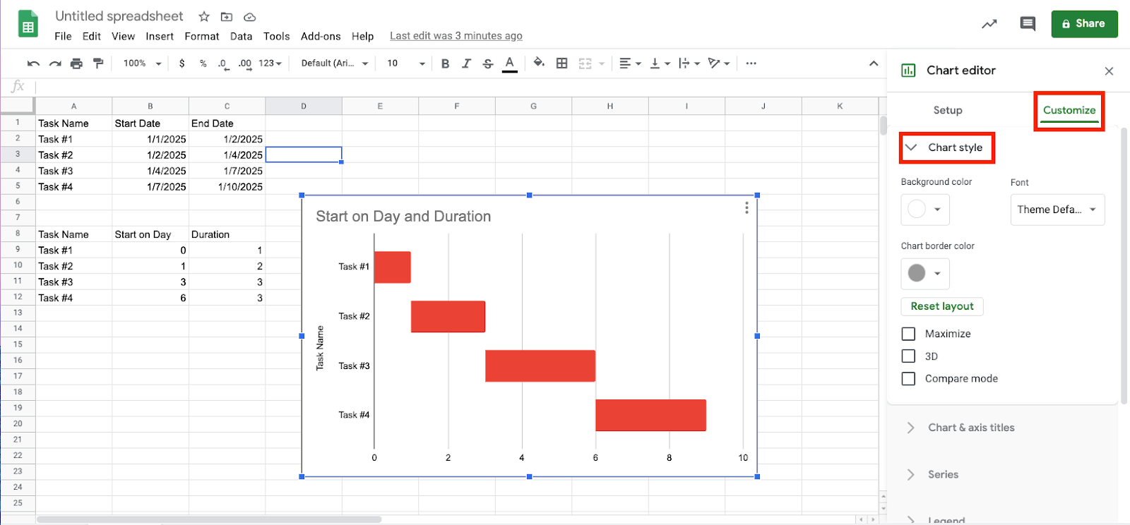
- Click on the chart and navigate to the Chart editor menu on the right.
- Click the Customize tab, then click the first option, Chart style.
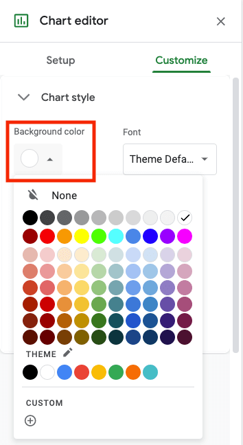
- Click the dropdown menu under Background color, then click a color to change the hue.
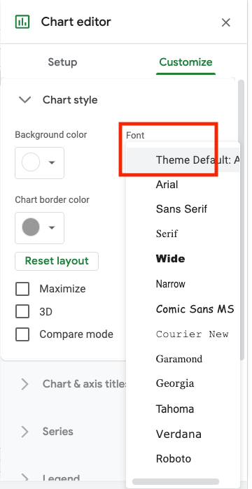
- Click on the text you want to change in the chart. Click the Font dropdown menu to change the font style for labels, legends, or the title.
Note: You will need to click on the text type to make changes.
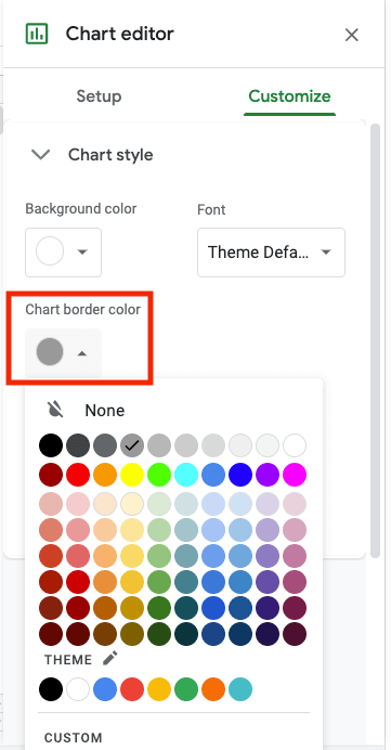
- Click the Chart border color dropdown menu. Click a border or color, or click None to remove it completely.
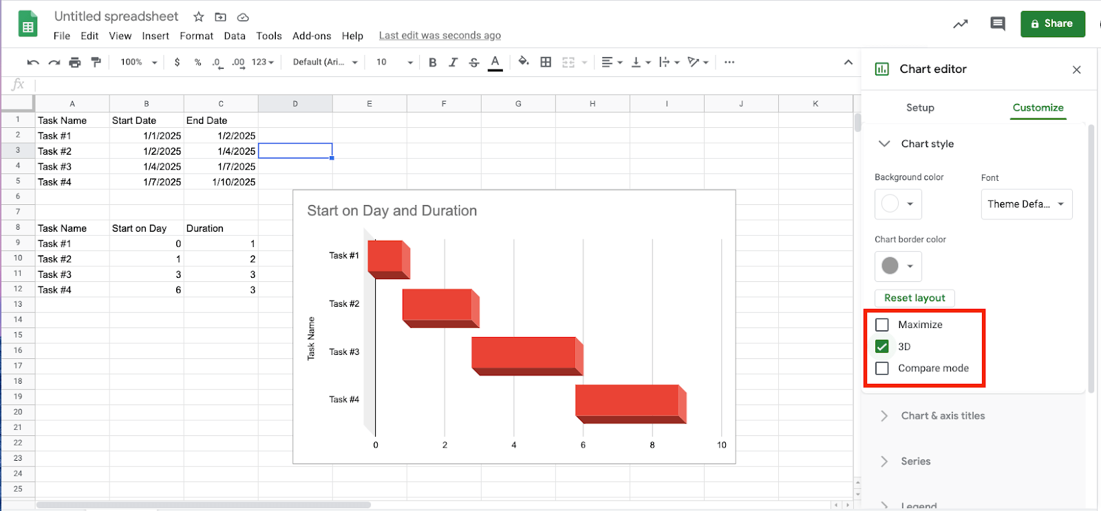
- Click the 3D box to add the effect to the bars.
Remove the Chart Legend from a Gantt Chart
- Click on the chart.
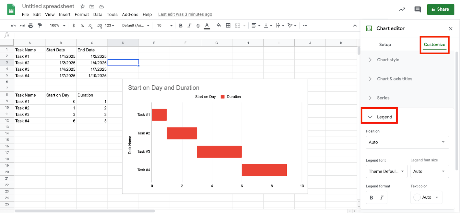
- Click the Customize tab in the Chart editor panel, then click Legend.
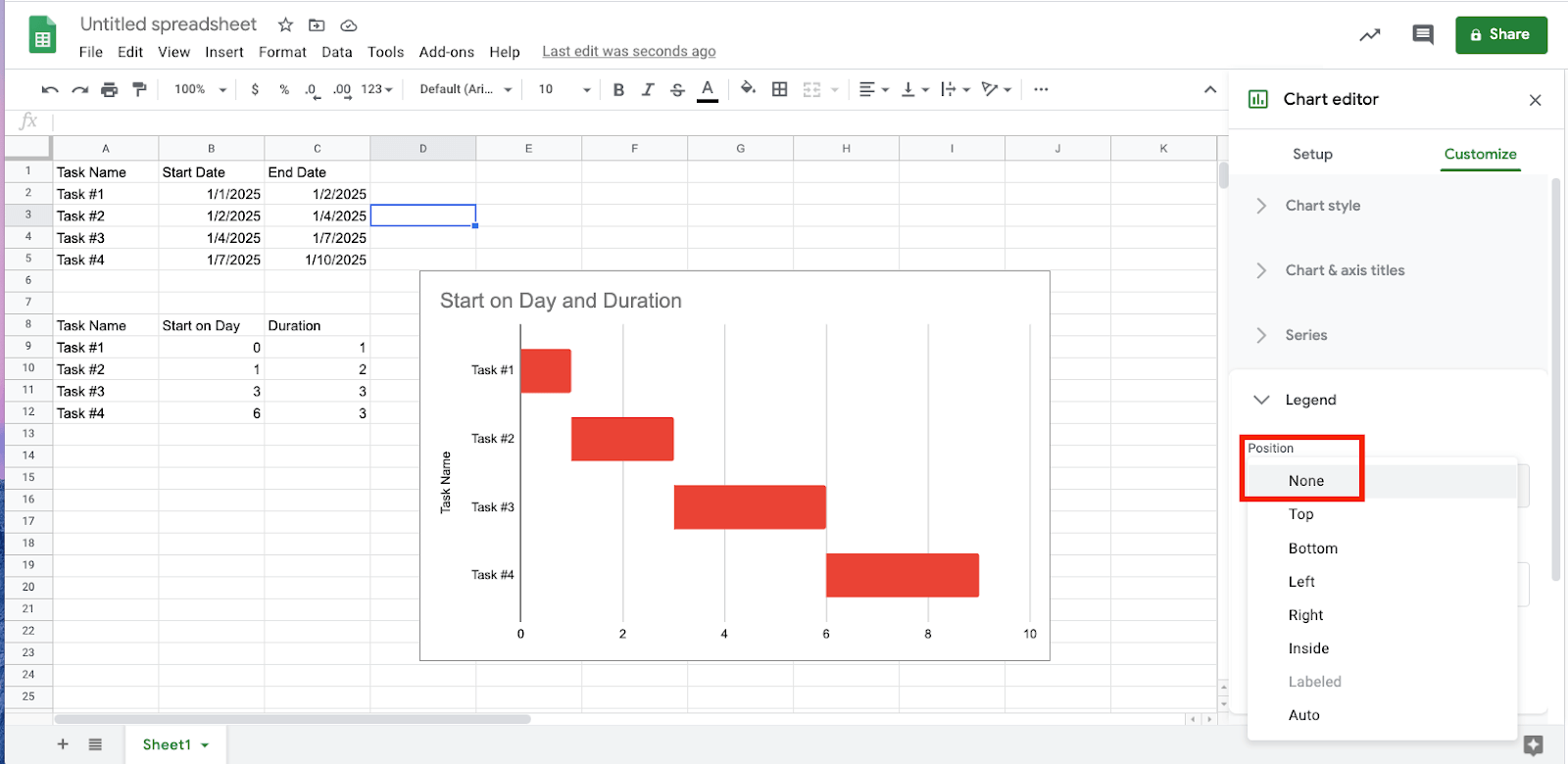
- Click the Position dropdown menu, then click None.
How to Handle Gantt Charts with Dependencies in Google Sheets
More complex projects will likely have project tasks that are dependent on one another — meaning, you can’t start some tasks until a previous task or series of tasks is complete. Follow these steps to ensure a dependent task does not start before the previous one is complete.
Set Up Dependent Tasks to Occur After Previous Tasks in a Gantt Chart
- Determine which tasks are dependent and the tasks they depend on.
- In the first table, click the cell of the dependent task (i.e., the task that cannot be started until a previous task is complete).
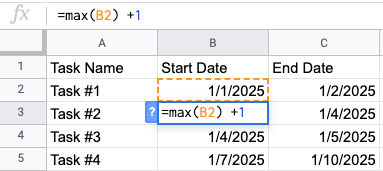
- In the Start Date cell of the dependent task, type in this formula:
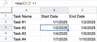
=max(B2)+1
Pro Tip: The values in this formula should be the tasks that must be completed before a dependent task can start. The +1 signifies this task can only start the day after the other tasks in the formula are completed.
- The resulting value in the dependent cell should be the date after the other tasks in the formula are projected to be completed.
Set Up Dependent Tasks to Occur Concurrently with Previous Tasks
With some projects, tasks need to happen simultaneously based on a predetermined timeline. Follow these steps to set up a system for tracking dependent tasks that happen concurrently with previous tasks.
- Determine which task(s) can run simultaneously.
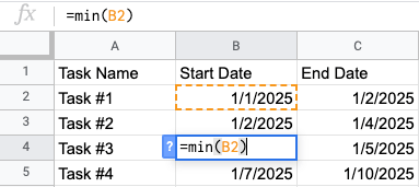
- Click the cell of the dependent task (in our example, cell B4) that you want to start on the same day as a previous task (in our example, cell B2).
- In the cell of the dependent task, type in this formula:
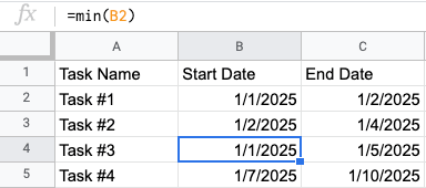
=min(B2)
Pro Tip: The values in this formula should be the tasks that you want to start at the same time as the dependent task. In this example, the task in cells B2 and B4 should be scheduled at the same time as the dependent task.
- The resulting value in the dependent cell should be the start date of the other tasks in the formula. In this case, Task #1 and Task #3 will show the same Start Date.
How to Export a Gantt Chart in Google Sheets to Excel
Some people prefer working in a more familiar spreadsheet interface, such as Microsoft Excel. Follow these steps to export a Gantt chart and all corresponding project data in Google Sheets to Excel.
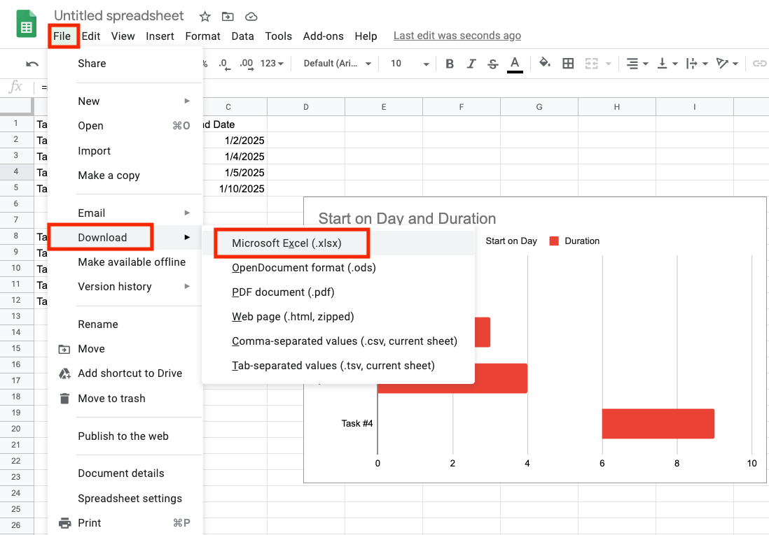
- Click File and scroll down to Download.
- From the Download dropdown menu, click Microsoft Excel (.xlsx).
Use this action to automatically create and download an Excel file.
Follow this tutorial to learn how to make a Gantt Sheet in Excel.
Gantt Chart Google Sheets Template
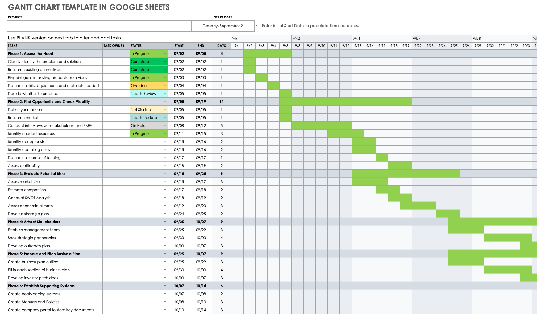
Track project progress, create dependent tasks, and visualize how each task is moving forward with this simple Gantt chart template in Google Sheets.
Download Gantt Chart Template - Google Sheets
Automatic Gantt Chart
Watch this short video to see how you can quickly turn a spreadsheet into a Gantt chart in a few easy steps using Smartsheet.
Dynamic Gantt Chart in Google Sheets
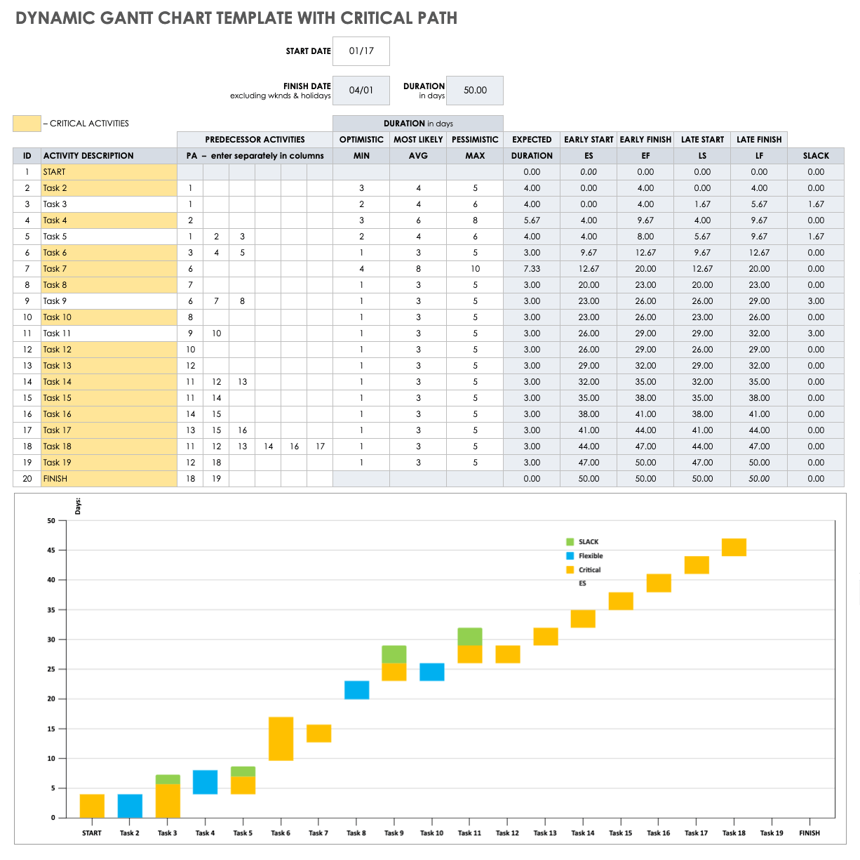
With this intricate Gantt chart template, you can not only track each project task as it moves along and plot dependencies on your chart, but you can also identify your project’s critical path. That way, you won’t miss key tasks in the process.
Download Dynamic Gantt Chart Template with Critical Path - Google Sheets
Peruse our collection of Gantt chart templates to find downloadable versions in other formats.
Get the Most Out of Your Gantt Charts with Smartsheet
Empower your people to go above and beyond with a flexible platform designed to match the needs of your team — and adapt as those needs change. The Smartsheet platform makes it easy to plan, capture, manage, and report on work from anywhere, helping your team be more effective and get more done. Report on key metrics and get real-time visibility into work as it happens with roll-up reports, dashboards, and automated workflows built to keep your team connected and informed. When teams have clarity into the work getting done, there’s no telling how much more they can accomplish in the same amount of time. Try Smartsheet for free, today.
